Active Learning : Maximal Expected Error Reduction
A programming introduction to Expected Error Reduction Query Strategy in Active Learning with State Vector Machine Model.


- Problem with Expected Model Change
- Main Idea 💡
- Experiment Configuration
- 2 Class Dataset
- Full DataFit
- Train, Pool, Test Split
- Fitting Model on Initial Train Data
- Calculating expected Future Loss
- Run Active Learning
- Plot Decision Boundaries
- References:
Problem with Expected Model Change
- Change in model parameters does not actually correspond to Model performance improvement
The next logical step we take is to directly focus on Performance metric , rather than to Model Change. So, we will choose the pool instance, which we expect would lead to most model improvement.
Main Idea 💡
Choose pool instance which Maximizes "generalization" Error Reduction once we add the instance to training set
We sort of use the pool instances as validation set.
But the pool instances are unlabelled, so we put an estimate to the error and look at expected error reduction.
Then we query the instance with minimal expected future error.
import numpy as np
import pandas as pd
import matplotlib.pyplot as plt
from matplotlib.animation import FuncAnimation
from matplotlib import animation
from matplotlib import rc
import matplotlib
from tqdm.notebook import tqdm
plt.style.use('fivethirtyeight')
rc('animation', html='jshtml')
colors = ['purple','green']
# To copy the models
from copy import deepcopy
# Sklearn Imports
from sklearn.linear_model import LogisticRegression
from sklearn.svm import SVC
from sklearn.datasets import make_classification, make_moons
from sklearn.model_selection import train_test_split
from sklearn.metrics import accuracy_score, f1_score
# Progress helper
from IPython.display import clear_output
class Config:
# Dataset Generation
n_features = 2
n_classes = 2
n_samples = 1000
dataset_random_state = 3
noise = 0.2
# Active Learning
test_frac = 0.2
init_train_size = 15
model_random_state = 0
active_learning_iterations = 50
# Saved GIF
fps = 8
# Base Model
n_jobs = 1
def get_base_model():
# return LogisticRegression(random_state = Config.model_random_state, n_jobs = Config.n_jobs)
return SVC(random_state = Config.model_random_state, probability=True)
X, y = make_classification(
n_samples=Config.n_samples,
n_features=Config.n_features,
n_informative=Config.n_features,
n_redundant=0,
n_classes=Config.n_classes,
random_state=Config.dataset_random_state,
shuffle=True,
)
plt.figure()
plt.scatter(X[:, 0], X[:, 1], c=y, cmap=matplotlib.colors.ListedColormap(colors))

model = get_base_model()
model.fit(X, y)
def plot_decision_surface(X, y, model):
grid_X1, grid_X2 = np.meshgrid(
np.linspace(X[:, 0].min() - 0.1, X[:, 0].max() + 0.1, 100),
np.linspace(X[:, 1].min() - 0.1, X[:, 1].max() + 0.1, 100),
)
grid_X = [(x1, x2) for x1, x2 in zip(grid_X1.ravel(), grid_X2.ravel())]
grid_pred = model.predict(grid_X)
plt.figure(figsize=(6, 5))
plt.scatter(X[:, 0], X[:, 1], c=y, cmap=matplotlib.colors.ListedColormap(colors))
plt.contourf(grid_X1, grid_X2, grid_pred.reshape(*grid_X1.shape), alpha=0.2, cmap=matplotlib.colors.ListedColormap(colors))
plot_decision_surface(X, y, model)

dataset_indices = list(range(len(X)))
train_pool_indices, test_indices = train_test_split(dataset_indices, test_size=Config.test_frac, random_state=0, stratify=y)
train_indices, pool_indices = train_test_split(train_pool_indices, train_size=Config.init_train_size, random_state=0)
indices_list = [train_indices, pool_indices, test_indices]
t_list = ['Train', 'Pool', 'Test']
fig, ax = plt.subplots(1,3,figsize=(15,4), sharex=True, sharey=True)
for i in range(3):
ax[i].scatter(X[indices_list[i]][:,0], X[indices_list[i]][:,1], c=y[indices_list[i]], cmap=matplotlib.colors.ListedColormap(colors))
ax[i].set_title(t_list[i])

AL_model = get_base_model()
AL_model.fit(X[train_indices], y[train_indices])
plot_decision_surface(X[train_indices], y[train_indices], AL_model)

Calculating expected Future Loss
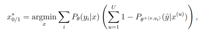
Expected 0/1 Loss is:
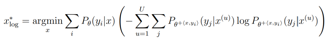
Expected Log-Loss is:
At each iteration:
For each unlabeled pool instance:
Suppose this instance is labeled and re-train the classifier adding this instance to training set
Re-infer the labels of remaining pool instances
Estimate the expected error on remaining pool instances
- In expected 0/1 loss, we use posterior probability of the most probable class
- In expected log loss, we use the posterior class distribution
End
Select the instance whose expected error reduction is largestdef query_expected_error_reduction(trn_indices, pl_indices, model, loss_type = "01"):
y_pred_proba = model.predict_proba(X[pl_indices])
expected_losses = []
# For each pool instance
for row_idx, pl_indx in enumerate(pl_indices):
new_temp_trn_X = X[trn_indices + [pl_indx]]
# Add pool instance to the training instance, assuming this class as the label
new_tmp_pl_indices = pl_indices.copy()
new_tmp_pl_indices.remove(pl_indx)
new_temp_pool_X = X[new_tmp_pl_indices]
expec_loss = 0
for clss in range(Config.n_classes):
new_temp_trn_y = np.append(y[trn_indices], clss)
clss_proba = y_pred_proba[row_idx][clss]
# Train the new model
new_temp_model = get_base_model()
new_temp_model.fit(new_temp_trn_X, new_temp_trn_y)
# Re-infer the remaining pool indices
new_tmp_y_pred_proba = new_temp_model.predict_proba(new_temp_pool_X)
new_tmp_y_pred_log_proba = new_temp_model.predict_log_proba(new_temp_pool_X)
new_tmp_y_pred = new_temp_model.predict(new_temp_pool_X)
new_tmp_y_pred_class_proba = new_tmp_y_pred_proba[range(len(new_tmp_pl_indices)), new_tmp_y_pred]
# Calculate expected loss
if loss_type == "01":
loss = np.sum(1 - new_tmp_y_pred_class_proba)
elif loss_type == "log":
loss = - np.sum(new_tmp_y_pred_proba * new_tmp_y_pred_log_proba)
else:
raise ValueError(f"{loss_type} not identified")
expec_loss += clss_proba * loss
expected_losses.append(expec_loss)
# Select instance with lowest expected error
return pl_indices[np.argmin(expected_losses)]
al_train_indices = train_indices.copy()
al_test_indices = test_indices.copy()
al_pool_indices = pool_indices.copy()
random_train_indices = train_indices.copy()
random_test_indices = test_indices.copy()
random_pool_indices = pool_indices.copy()
AL_models = []
random_models = []
AL_added_indices = []
random_added_indices = []
np.random.seed(0)
for active_iteration in tqdm(range(Config.active_learning_iterations)):
##### Maximal Expected Error Reduction Strategy ######
# Fit model
AL_model = get_base_model()
AL_model.fit(X[al_train_indices], y[al_train_indices])
AL_models.append(deepcopy(AL_model))
# Query a point
query_idx = query_expected_error_reduction(al_train_indices, al_pool_indices, AL_model, loss_type = "01")
AL_added_indices.append(query_idx)
# Add query index to train indices and remove from pool indices
al_train_indices.append(query_idx)
al_pool_indices.remove(query_idx)
##### Random Strategy #####
# Fit model
random_model = get_base_model()
random_model.fit(X[random_train_indices], y[random_train_indices])
random_models.append(deepcopy(random_model))
# Query a point
query_idx = np.random.choice(random_pool_indices)
random_added_indices.append(query_idx)
# Add query index to train indices and remove from pool indices
random_train_indices.append(query_idx)
random_pool_indices.remove(query_idx)
X_test = X[test_indices]
y_test = y[test_indices]
random_scores = []
AL_scores = []
for iteration in range(Config.active_learning_iterations):
clear_output(wait=True)
print("iteration", iteration)
AL_scores.append(accuracy_score(y_test, AL_models[iteration].predict(X_test)))
random_scores.append(accuracy_score(y_test, random_models[iteration].predict(X_test)))
plt.plot(AL_scores, label='Active Learning, 0/1 Loss')
plt.plot(random_scores, label='Random Sampling')
plt.legend()
plt.xlabel('Iterations')
plt.ylabel('Accuracy\n(Higher is better)')

grid_X1, grid_X2 = np.meshgrid(
np.linspace(X[:, 0].min() - 0.1, X[:, 0].max() + 0.1, 100),
np.linspace(X[:, 1].min() - 0.1, X[:, 1].max() + 0.1, 100),
)
grid_X = [(x1, x2) for x1, x2 in zip(grid_X1.ravel(), grid_X2.ravel())]
X_train, y_train = X[al_train_indices], y[al_train_indices]
X_train_rand, y_train_rand = X[random_train_indices], y[random_train_indices]
def update(i):
for each in ax:
each.cla()
AL_grid_preds = AL_models[i].predict(grid_X)
random_grid_preds = random_models[i].predict(grid_X)
# Active learning
ax[0].scatter(X_train[:n_train,0], X_train[:n_train,1], c=y_train[:n_train], label='initial_train', alpha=0.2, cmap=matplotlib.colors.ListedColormap(colors))
ax[0].scatter(X_train[n_train:n_train+i, 0], X_train[n_train:n_train+i, 1],
c=y_train[n_train:n_train+i], label='new_points', cmap=matplotlib.colors.ListedColormap(colors))
ax[0].contourf(grid_X1, grid_X2, AL_grid_preds.reshape(*grid_X1.shape), alpha=0.2, cmap=matplotlib.colors.ListedColormap(colors))
ax[0].set_title('New points')
ax[1].scatter(X_test[:, 0], X_test[:, 1], c=y_test, label='test_set', cmap=matplotlib.colors.ListedColormap(colors))
ax[1].contourf(grid_X1, grid_X2, AL_grid_preds.reshape(*grid_X1.shape), alpha=0.2, cmap=matplotlib.colors.ListedColormap(colors))
ax[1].set_title('Test points')
ax[0].text(locs[0],locs[1],'Active Learning')
# Random sampling
ax[2].scatter(X_train_rand[:n_train,0], X_train_rand[:n_train,1], c=y_train_rand[:n_train], label='initial_train', alpha=0.2, cmap=matplotlib.colors.ListedColormap(colors))
ax[2].scatter(X_train_rand[n_train:n_train+i, 0], X_train_rand[n_train:n_train+i, 1],
c=y_train_rand[n_train:n_train+i], label='new_points', cmap=matplotlib.colors.ListedColormap(colors))
ax[2].contourf(grid_X1, grid_X2, random_grid_preds.reshape(*grid_X1.shape), alpha=0.2, cmap=matplotlib.colors.ListedColormap(colors))
ax[2].set_title('New points')
ax[3].scatter(X_test[:, 0], X_test[:, 1], c=y_test, label='test_set', cmap=matplotlib.colors.ListedColormap(colors))
ax[3].contourf(grid_X1, grid_X2, random_grid_preds.reshape(*grid_X1.shape), alpha=0.2, cmap=matplotlib.colors.ListedColormap(colors))
ax[3].set_title('Test points')
ax[2].text(locs[0],locs[1],'Random Sampling')
locs = (2.7, 4)
fig, ax = plt.subplots(2,2,figsize=(12,6), sharex=True, sharey=True)
ax = ax.ravel()
n_train = X_train.shape[0] - Config.active_learning_iterations
anim = FuncAnimation(fig, func=update, frames=range(Config.active_learning_iterations))
plt.close()
anim
mywriter = animation.PillowWriter(fps=Config.fps)
anim.save('./assets/2022-02-22-maximal-expected-error-reduction-active-learning/active-learning.gif',writer=mywriter)
Major Drawbacks:
- Very expensive: In each active learning iteration, we have to incrementally re-train the model by adding a new pool instance. Therefore in each iterations, we re-train the model $n\_classes \times n\_pool$ times, which is very expensive.
The computational cost is linear to the number of classes and number of pool instances.
In most cases, it is the most computationally expensive query framework.
References:
- Active Learning Literature Survey by Burr Settles, Section 3.4
- YouTube :: Lecture 26 Active Learning for Network Training: Uncertainty Sampling and other approaches by Florian Marquardt
- Original Maximal EER paper.Toward Optimal Active Learning through Sampling Estimation of Error Reduction by Roy and McCallum. ICML, 2001.